Code
source("../appendix/packages.R")
source("../appendix/feature_labels.R")source("../appendix/packages.R")
source("../appendix/feature_labels.R")This chapter provides an overview of the concepts and methodologies analysed in this research. It provides a brief introduction to remote sensing, machine learning techniques, and their applications in land cover mapping and SDG monitoring.
# data for the number of satellites
UCS_Satellite_Database <- read.csv("figures/UCS-Satellite-Database_5-1-2023.csv")

UCS_Satellite_Database_EarthObs <-
  UCS_Satellite_Database |>
  mutate(Date_Launch = as.Date(Date_Launch, format = "%Y-%m-%d"))|>
  filter(!grepl("Military", Users))|>
  filter(grepl("Earth",Purpose ))

prop_after_2020<- sum(year(UCS_Satellite_Database_EarthObs$Date_Launch)>=2020,
                      na.rm = TRUE)/ nrow(UCS_Satellite_Database_EarthObs)
In the broadest sense, remote sensing involves acquiring information about an object or phenomenon without direct contact (Campbell & Wynne, 2011). More specifically, remote sensing refers to gathering data about land or water surfaces using sensors mounted on aerial or satellite platforms that record electromagnetic radiation reflected or emitted from the Earth’s surface (Campbell & Wynne, 2011, p. 6). The origins of remote sensing lie with the development of photography in the 19th century, with the earliest aerial or Earth Observation photographs taken with cameras mounted on balloons, kites, pigeons, and aeroplanes. (Burke et al., 2021; Campbell & Wynne, 2011, p. 7). The first mass use of remote sensing was during World War I with aerial photography. The modern era of satellite-based remote sensing started with the launch of Landsat 1 in 1972, the first satellite specifically designed for Earth Observation (Campbell & Wynne, 2011, p. 15). Today, remote sensing technology enables frequent and systematic collection of data about the Earth’s surface with global coverage, revolutionizing our ability to monitor and analyze the Earth’s surface (Burke et al., 2021; NASA, 2019). As of May 2023, roughly 1039 active nonmilitary Earth Observation satellites are in orbit; 51% were launched in 2020 (UCS, 2021).
ggplot(data = UCS_Satellite_Database_EarthObs|>
         group_by(week = lubridate::floor_date(Date_Launch, 'week'))|>
         summarise(n = n()),
       aes(x = week, y = n)) +
  geom_line(aes(y = cumsum(n)), na.rm = TRUE) +

  scale_x_date(date_breaks = "5 years", date_labels = "%Y") +

  labs(y = "Number of Satellite", x = "Year",
        title = "Number of Satellites Launched Over Time") +
  common_theme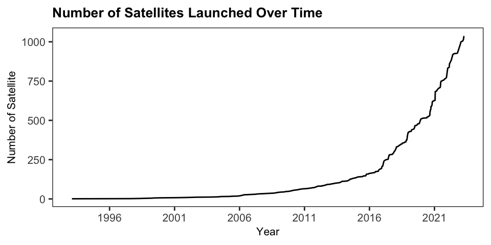
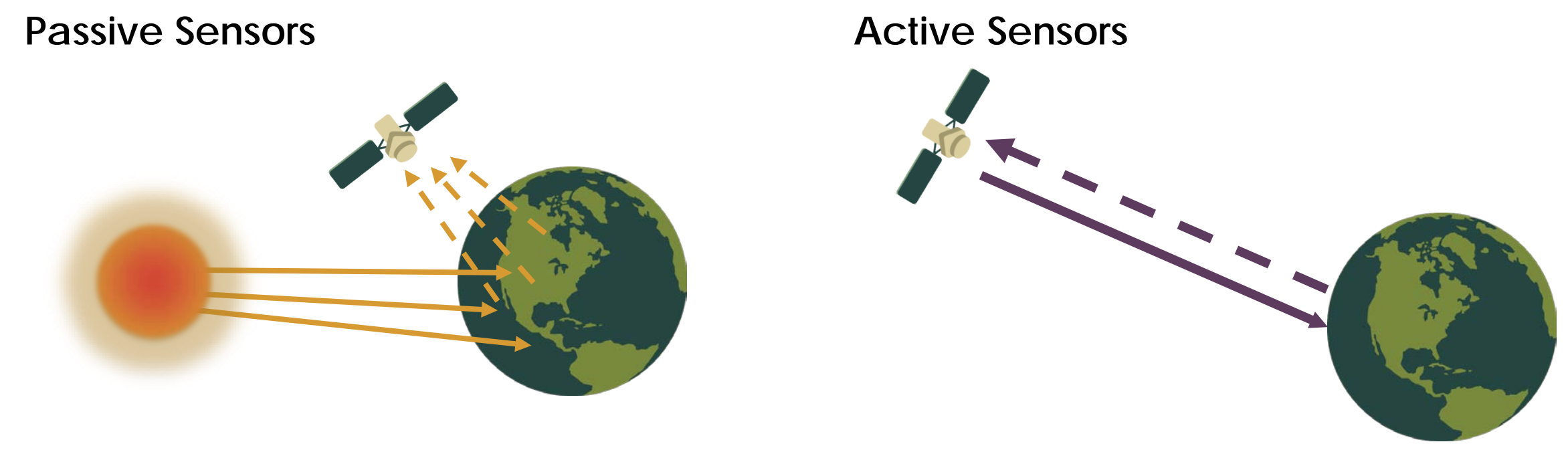
Sensors on remote sensing devices such as satellites measure electromagnetic radiation reflected by objects on the Earth’s surface. This is done in two different ways: passive and active. Passive sensors rely on natural energy sources, like sunlight, to record incident energy reflected off the Earth’s surface. While active sensors generate their own energy, which is emitted and then measured as it reflects back from with the Earth’s surface (NASA, 2019).
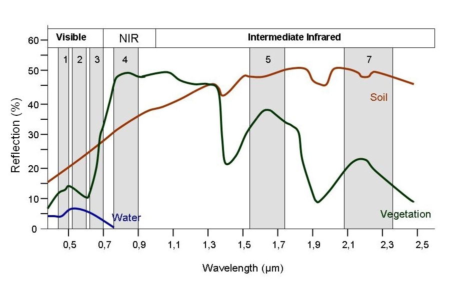
Components of the Earth’s surface have different spectral signatures — i.e., reflect, absorb, or transmit energy in different amounts and wavelengths (Campbell & Wynne, 2011). Remote sensing devices have several sensors that measure specific ranges of wavelengths in the electromagnetic spectrum; these are referred to as spectral bands; e.g., visible light, infrared, or ultraviolet radiation (NASA, 2019; SEOS, 2014). By capturing information from particular bands, the spectral signatures of surfaces can be used to identify objects on the ground. Figure 2.3 illustrates the differences between the spectral signatures of soil, green vegetation, and water across various wavelengths. The grey bands in the figure represent the specific spectral bands on the Landsat TM satellite (SEOS, 2014). The distinct reflectance properties of each material within these bands enable the differentiation of surface materials, making it possible to identify different land cover types. This information can be used directly for classification, or it can be combined into indices—such as the Normalized Difference Vegetation Index (NDVI)—to enhance the detection of specific features like vegetation health and coverage (Campbell & Wynne, 2011; NASA, 2019). The \(NDVI\) uses red light and near-infrared (NIR) to distinguish green vegetation. Higher \(NDVI\) values indicate green vegetation as more red light is absorbed, whereas lower values correspond to non-vegetated areas where more red light is reflected.
Machine learning techniques such as neural networks, random forests, and support vector machines have long been applied for spatial data analysis and geographic modelling (Haddaway et al., 2022; Lavallin & Downs, 2021). Compared to using indices alone, machine learning techniques enhance the accuracy and efficiency of data analysis and interpretation processes, making it possible to analyze large volumes of data effectively. This is particularly useful for handling the high complexity and dimensionality of remote sensing data. In recent years, the application of machine learning techniques in remote sensing has surged, driven by the increasing availability of large datasets and advancements in computational power (UN-GGIM:Europe, 2019; Y. Zhang et al., 2022).
These machine learning models can be grouped into four main types according to the aims of analyses: classification, clustering, regression, and dimension reduction. Table 2.1 describes this grouping and gives examples. It is important to note that recent trends in machine learning and remote sensing analyses use hybrid or ensemble approaches using a combination of these groups, for a thorough review of these methods see UN-GGIM:Europe (2019).
read_excel("figures/summary_tables.xlsx", sheet = "ML_cat")|>
  kable(booktabs = TRUE, linesep = "") |>
  kable_styling(font_size = 10,
                full_width = FALSE)|>
  column_spec(1, width = "2cm")|>
  column_spec(2, width = "14cm")|>

  footnote(c("Adapted from UN-GGIM:Europe (2019) and Haddaway et al.(2022)."),
threeparttable=TRUE)| Analysis aim | Explanation |
|---|---|
| Classification | Assigning objects to known classes based on input variables. For example, categorizing pixels in an image into crop types using a model trained on known data. |
| Regression | Predict a numeric (discrete or continuous) response variable based on input variables, similar to classification but with numeric outputs. An example is predicting crop yield from Earch Observation image data. |
| Clustering | Groups objects based on input variables without pre-defined classes, identifying similarities among the objects. This can help in grouping pixels in an image for further inspection. |
| Dimension reduction | Reduces a large set of variables to a smaller set that retains most of the original information. This can simplify analysis or generate new variables like indices (e.g., Vegetation Index) for interpretation. |
| Note: | |
| Adapted from UN-GGIM:Europe (2019) and Haddaway et al.(2022). |
Performance metrics are used to verify these analyses, which for classification tasks involve creating a confusion matrix — a cross-tabulation of class labels assigned to model predictions and reference data (ground truth). In a confusion matrix, the correctly classified instances are on the diagonal, and the off-diagonal cells indicate which classes are confused (i.e., incorrectly classified). In remote sensing applications, accuracy assessments are undertaken on a pixel, group of pixels (e.g. block), or an object level (Stehman & Foody, 2019).
confusion <- data.frame(
  Reference = c("Class 1","Class 2","Class 3","Class 4", "Total", "User's accuracy"),
  #Predictions
  c1 = c("$m_{11}$", "$m_{21}$", "$m_{31}$", "$m_{41}$", "$m_{.1}$", "$m_{11}/m_{.1}$"),
  c2 = c("$m_{12}$", "$m_{22}$", "$m_{32}$", "$m_{42}$", "$m_{.2}$", "$m_{22}/m_{.2}$"),
  c3 = c("$m_{13}$", "$m_{23}$", "$m_{33}$", "$m_{43}$", "$m_{.3}$", "$m_{33}/m_{.3}$"),
  c4 = c("$m_{14}$", "$m_{24}$", "$m_{33}$", "$m_{44}$", "$m_{.4}$", "$m_{44}/m_{.4}$"),
  total = c("$m_{1.}$", "$m_{2.}$", "$m_{3.}$", "$m_{4.}$", "$m$", ""),
  pa = c("$m_{11}/m_{1.}$", "$m_{22}/m_{2.}$",
         "$m_{33}/m_{3.}$", "$m_{44}/m_{4.}$", "", "")
)
confusion|>
  kable(booktabs = TRUE, linesep = "", escape = FALSE,
        col.names = c("Reference","Class 1","Class 2","Class 3","Class 4", "Total", "Producer's accuracy")
        ) |>
  kable_styling(font_size = 10,
                full_width = FALSE)|>
  add_header_above(c("", "Predictions" = 6), bold = TRUE) |>
  row_spec(0, bold = TRUE)|>
  column_spec(1, bold = TRUE)|>
  footnote(c("The rows ($r$) represent the reference (observed) classification and the columns ($c$) represent the predicted classes. $m_{rc}$ is the number of instances in reference (observered) class $r$ and predicted class $c$, and $m$ is the total number of instances (i.e., the number of pixels/objects classified)."),
threeparttable=TRUE, escape=FALSE)| Reference | Class 1 | Class 2 | Class 3 | Class 4 | Total | Producer's accuracy |
|---|---|---|---|---|---|---|
| Class 1 | $m_{11}$ | $m_{12}$ | $m_{13}$ | $m_{14}$ | $m_{1.}$ | $m_{11}/m_{1.}$ |
| Class 2 | $m_{21}$ | $m_{22}$ | $m_{23}$ | $m_{24}$ | $m_{2.}$ | $m_{22}/m_{2.}$ |
| Class 3 | $m_{31}$ | $m_{32}$ | $m_{33}$ | $m_{33}$ | $m_{3.}$ | $m_{33}/m_{3.}$ |
| Class 4 | $m_{41}$ | $m_{42}$ | $m_{43}$ | $m_{44}$ | $m_{4.}$ | $m_{44}/m_{4.}$ |
| Total | $m_{.1}$ | $m_{.2}$ | $m_{.3}$ | $m_{.4}$ | $m$ | |
| User's accuracy | $m_{11}/m_{.1}$ | $m_{22}/m_{.2}$ | $m_{33}/m_{.3}$ | $m_{44}/m_{.4}$ | ||
| Note: | ||||||
| The rows ($r$) represent the reference (observed) classification and the columns ($c$) represent the predicted classes. $m_{rc}$ is the number of instances in reference (observered) class $r$ and predicted class $c$, and $m$ is the total number of instances (i.e., the number of pixels/objects classified). |
From this matrix, performance measures such as overall accuracy are derived (FAO, 2016; Stehman & Foody, 2019; UN-GGIM:Europe, 2019) where the overall accuracy is the total number of successful classifications \(s\) over the total number of instances, \(m\) (\(q\) is the number of classes).
\[ \text{Overall Accuracy (OA)} = \frac{\sum^q_{r=1}m_{rr}}{m}= \frac{s}{m} \tag{2.1}\]
If the unit of accuracy assessment is a pixel, then overall accuracy is the proportion of pixels classified correctly. Other metrics include reliability (User’s accuracy) and sensitivity (recall or Producer’s accuracy). Reliability is the correct classification for a particular class divided by the column total (\(m_{.c}\)), and sensitivity is the correct classification over the row total (\(m_{r.}\)). It is important to consider the map’s purpose when evaluating its accuracy, as overall accuracy may not reflect the accuracy of specific classes. Factors such as sample size, class stability, class proportions, and landscape variability influence the overall accuracy (FAO, 2016; see UN-GGIM:Europe, 2019).
As an example of how remote sensing data and machine learning can be used to support ecologically sustainable development, Owers et al. (2022) developed an approach to monitor and map land cover across Australia using techniques. Their study used Landsat sensor data archive through Digital Earth Australia to generate annual land cover maps from 1988 to 2020 at a 25-meter resolution. The study used random forest and artificial neural networks to classify individual pixels according to the FAO’s Land Cover Classification System (LCCS) framework.
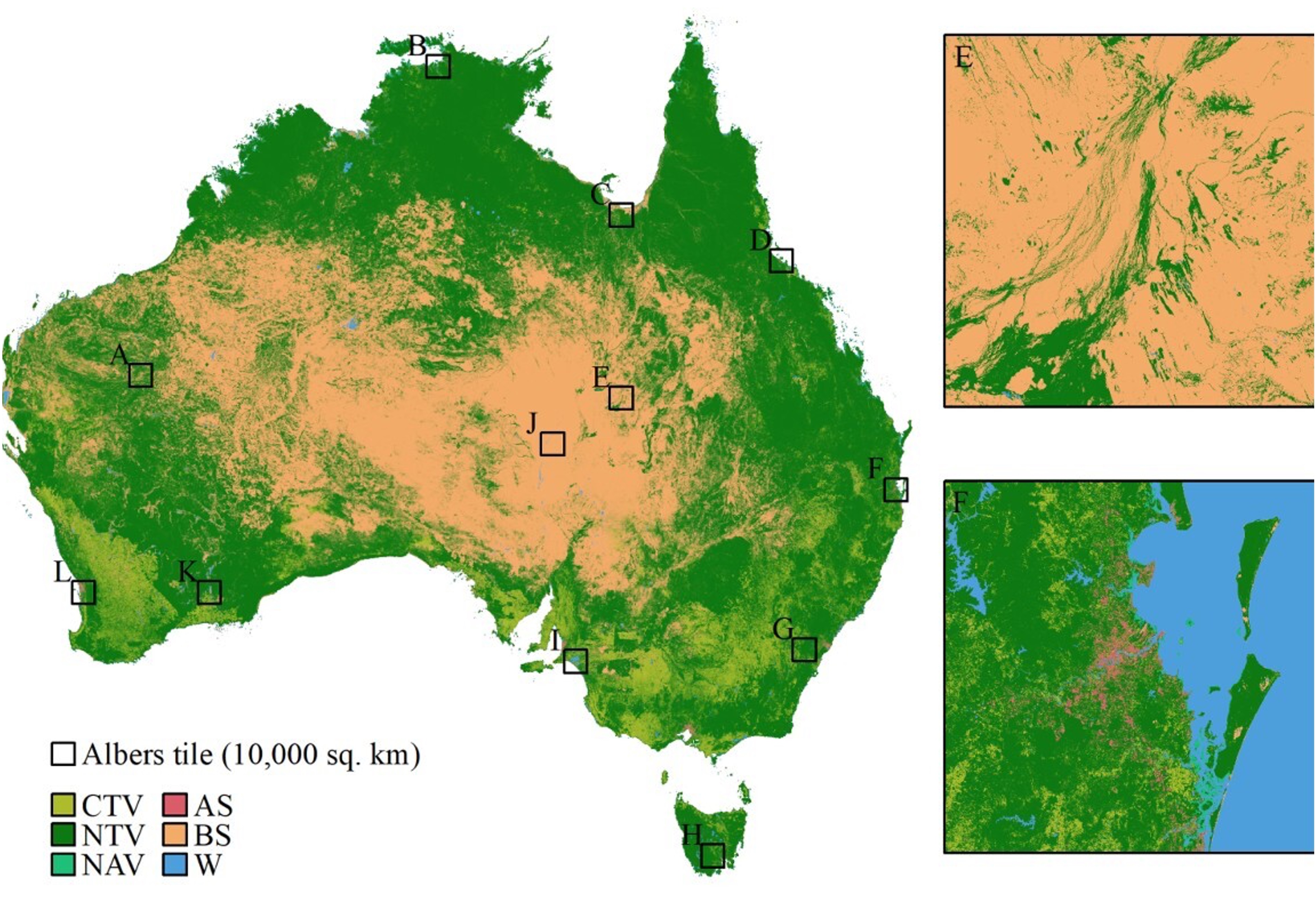
Producing such detailed maps through traditional topographical field surveys would be impractical, given Australia’s size (\(7,688,287 \text{ km}^2\)). While field surveys are considered the most accurate method for generating training sample data, they are labor-intensive, time-consuming, and costly (C. Zhang & Li, 2022). For example, surveying just 20 hectares (\(0.2 \text{ km}^2\)) would take a team of four people approximately five days to complete, though the resulting topographical map would have a high resolution of 0.5 meters (L.A. Mbila, personal communication, January 26, 2024). In Owers et al. (2022), experts visually inspected the satellite imagery to validate the training and test data. While this method is less labor-intensive, costly, and time-consuming than field surveys, it still demands significant effort and expertise.
In contrast to the limitations of field surveys, remote sensing provides an efficient means for continuously monitoring large, often inaccessible areas (Owers et al., 2022; C. Zhang & Li, 2022). The potential applications of this technology are vast, including land use and degradation monitoring, forestry, biodiversity assessment, agriculture, disaster prediction, water resource management, public health, urban planning, poverty tracking, and the management and preservation of world heritage sites (Anshuka et al., 2019; Campbell & Wynne, 2011; Ekmen & Kocaman, 2024; O. Hall et al., 2023; Lavallin & Downs, 2021; Maso et al., 2023).
Numerous studies have previously examined the application of remote sensing for SDG monitoring. However, existing reviews are typically either limited to specific contexts, such as the use of satellite data for poverty estimation (O. Hall et al., 2023) or focus on descriptive results (see Yin et al., 2023). The existing reviews either apply methodology that aligns more closely with Synthesis Without Meta-Analysis (Campbell et al., 2020) —for example, Thapa et al. (2023) and Ekmen & Kocaman (2024) — or apply unweighted meta-analysis techniques, such as Khatami et al. (2016) and O. Hall et al. (2023). In an unweighted meta-analysis all studies are treated equally regardless of their sample size, quality, or variance (J. A. Hall & Rosenthal, 2018). However, it is more common in traditional applications of meta-analysis, to use the sample sizes when aggregating individual studies (J. A. Hall & Rosenthal, 2018). However, to my knowledge, no examples of a weighted meta-analysis applied to predictive performance in remote sensing data have been conduced, highlighting a gap that this study aims to address.