The analysis on this dashboard updates daily (at 12:00 CET). Users can make contribute to the data for this analysis and see how it affects the results. For information on how to add to the dataset see Contribute data page. The table bellow shows the data collected columns are added by contributor.
| Feature | nina_2024, N = 86 | test, N = 1 |
|---|---|---|
| Overall Accuracy | 0.90 (0.65 - 1.00) | 0.90 (0.90 - 0.90) |
| Sample Size | 6,401,352 (259 - 75,782,016) | 100 (100 - 100) |
| Majority-class Proportion | 0.72 (0.14 - 1.00) | 0.90 (0.90 - 0.90) |
| Ancillary Data | ||
| Ancillary Data Included | 15 (17%) | 0 (0%) |
| Remote Sensing Only | 71 (83%) | 1 (100%) |
| Indices | ||
| Not Used | 23 (27%) | 0 (0%) |
| Used | 63 (73%) | 1 (100%) |
| Number of Spectral Bands | ||
| Low | 16 (19%) | 0 (0%) |
| Mid | 28 (33%) | 0 (0%) |
| Not Reported | 42 (49%) | 1 (100%) |
| Confusion Matrix | ||
| Not Reported | 23 (27%) | 0 (0%) |
| Reported | 63 (73%) | 1 (100%) |
| Model Group | ||
| NN | 41 (48%) | 0 (NA%) |
| Other | 4 (4.7%) | 0 (NA%) |
| RF | 36 (42%) | 0 (NA%) |
| SVM | 5 (5.8%) | 0 (NA%) |
| Unknown | 0 | 1 |
| Note: | ||
| Mean (Min - Max); n(%) |
The fit model for this analysis is a multilevel meta-regression using the rma.mv function from the metafor package. This model allows for a random-effects meta-regression, where the goal is to account for variability both within and between studies. The model here is:
\[\text{overall accuracy}_{_{transformed}} = \text{proportion majority class + ancillary + indices + confusion matrix + model group}\]
The table bellow shows the heterogeneity in the overall accuracy from the dataset, both with and without study features. Heterogeneity is a measure of the variability in effect sizes across studies, and it helps to understand the extent to which the included studies are similar or different from one another.
Without- |
With- study features |
||||||||||||
|---|---|---|---|---|---|---|---|---|---|---|---|---|---|
| $\sigma^2_{\text{level2}}$ | $\sigma^2_{\text{level3}}$ | $\sigma^2_{\text{level2}}$ | $\sigma^2_{\text{level3}}$ | $Q_E$ | df | $p_Q$ | $F$ | df | $p_F$ | $I^2_{\text{level2}}$ | $I^2_{\text{level3}}$ | $R^2_{\text{level2}}$ | $R^2_{\text{level3}}$ |
| 0.01 | 0.017 | 0.009 | 0.006 | 11369118 | 76 | 0 | 4 | 9 | 0.018 | 60.53 | 39.47 | 6.3 | 63.8 |
Without Study Features: This column shows the heterogeneity estimates when no study features are considered. With Study Features: This column indicates the heterogeneity estimates when study features (model defined above) are included in the analysis. The metrics included are:
\(\sigma^2\) The variance estimates at different levels (level 2: within- and level 3: between- study).
Q and p-values: Test statistics for heterogeneity, where a significant p-value (\(p_Q\)) suggests significant heterogeneity.
\(I^2\): The percentage of variability due to heterogeneity rather than chance.
\(R^2\): The proportion of variance explained by the model.
The coefficient table shows the impact of each study feature on the overall accuracy. Positive or negative values indicate the direction and magnitude of the effect for each feature. It is important to note that the results shown are in a transformed scale and may not have the same interpretation when back-transformed
Feature Name: Each row represents a study feature.
Estimate: The coefficient (or beta) for each feature, representing the strength and direction of its influence.
Standard Error: The standard deviation of the coefficient, which helps understand the uncertainty around the estimate.
p-value: This indicates whether the feature is statistically significant. If the p-value is less than 0.05, the feature likely has a meaningful impact on the heterogeneity.
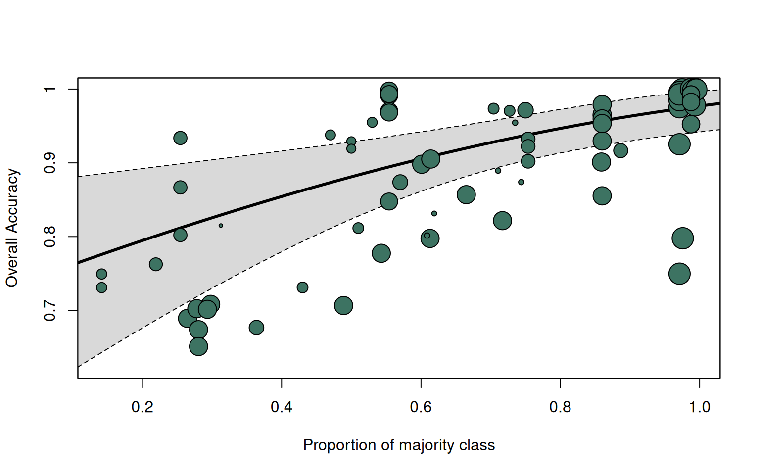
To visualize the relationship between the proportion of majority class and overall accuracy. Each bubble represents a result from a study, with the size of the bubble indicating the study’s weight or sample size.